CSIM - Parallel Process and Diagrams Simulator
admin@csim.com
Contents
- Introduction
-
1.1 Simple Example
- Topology Description
- Behavioral Description
-
3.1 Variable Scoping Levels
3.2 Standard Pre-defined Variables
3.3 Thread C-Code: DELAY, SEND, RECEIVE, TRIGGER_THREAD, CHECK_IN_PORT_QUEUE
3.4 Example Behavioral Description
3.5 Local Subroutines
3.6 Global Definitions
3.7 Include Directive
3.8 CSIM_PRINTF and CSIM_ANNOUNCE
3.9 RECEIVE_IR, RECEIVE_ALL_PORTS, and RECEIVE_ANY
3.10 Preempting or Re-scheduling Future Events
3.11 Animation Highlighting
3.12 Annotation Animation
3.13 Synchrons: WAIT, RESUME, WAIT_WITH_TIMEOUT, SCHEDULE_RESUME_WITH_PARAM
3.14 Halt and CSIM_HALT_POPUP
3.15 Conditional Model Inclusion (%ifdef, %ifndef, %define)
3.16 Thread Exit
3.17 Model Attributes
3.18 Model Aliases
- Simulator Usage
- Appendix A - Text format of topology file
- Appendix B - Warning and Error Messages Explained
- Appendix C - Gauge Display Gadget
- Appendix D - XY-Graph Display Gadget
- Appendix E - User Buttons Gadget
- Appendix F - User Text-Entry Gadget
- Appendix G - User Slider-Control Gadget
- Appendix H - Command-line options
- Appendix I - Listing Ports
- Appendix J - Image-Icons, and Icon Animations
- Appendix K - Accessing Command-Line Arguments
- Appendix L - Instance Attributes
- Appendix M - Setting Animation Modes
- Appendix N - Detecting End of Simulation - CSIM_EndOfSim
- Appendix O - Animating DFG's
- Appendix P - Pop-Up Messages From Models
- Appendix Q - Bar-Chart and Strip-Chart Gadgets
- Appendix R - Registering Event-loop & Exit Functions
1.0 Introduction:
The CSIM environment consists of a set of tools for describing parallel systems, for running simulations, and for viewing simulation results. Additionally, several model libraries have been developed for use with CSIM.The CSIM simulator is the core tool in the tool set. CSIM is a discrete event simulator for describing parallel processor architectures and software mappings. This document describes the CSIM simulator and the formats for its data files. The related tools and libraries are documented separately.
CSIM is intended for:
- Quickly describing the behavior of each type of device in a multi-device system in terms of time delays, functions, and interactions with other devices through designated ports.
- Quickly interconnecting the models described in (A) according to arbitrarily described topologies and running discrete event simulations of the described system.
- Using (A) and (B) for investigating the effects of link bandwidth in conjunction with network architecture. (buses, rings, meshes, etc.), and for investigating the time related performance of algorithm mappings onto the modeled architectures.
The CSIM input consists of two parts:
- The system structural topology (produced by the GUI or a text editor),
- The device-type behavior descriptions. (referenced from library or produced by a text editor).
Because the device models are written in standard C-language, CSIM simulations are flexible and efficient. Models may be as abstract or detailed as C allows, and any sort of statistics may be easily described and collected. Anything that can be called or done from C-code can be done in CSIM.
Although a CSIM simulation is executed on a single workstation, CSIM creates the illusion that the modeled devices are executing concurrently.
Under CSIM, C-language descriptions of the behavior of each device type, such as a processor node, can be written as if it would be compiled and run on that node with no notion of other devices in the system other than at the SEND/RECEIVE communication points. The SEND/RECEIVE calls are blocking. This means that, if no data has arrived, the code executing the RECEIVE call will hold until data arrives. Similarly, if an attempt to send data is made when the output buffer has reached its specified capacity, the sending process holds-up until the receiving device accepts some data.
Although a given device may hold, simulation time continues to advance, and events in other devices continue to occur. Computation delays can be modeled by placing a DELAY( xx-us ); statement in the model code.
The time required for data to be transferred across inter-device links depends on the link data-rate (specified in the topology) and the amount of data sent (specified in the SEND call). Since data is transferred only at the rate specified for a given link, even if an attempt is made to send many messages simultaneously, each will not arrive until the appropriate time has elapsed to transfer the prior messages. In other words, link bandwidth is automatically enforced by CSIM.
1.1 Simple Example:
The following is a VERY simple example of a CSIM model of a system that contains only two devices. Figure 1.1 shows the structure of the system as entered by the CSIM GUI. It shows the topology and devices of the modeled system. Each of the two devices is of the same type, so only one type of device need be described. It is instantiated twice.
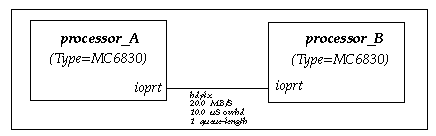
Figure 1.1 - Topology of simple example system.
Figure 1.2 - Behavior of simple example device-type.
 (Table of Contents.)
2.0 Topology Description:
The topology description is a block diagram that describes how blocks are connected to each other. Such descriptions are sometimes called, structural, or architectural descriptions. The topology shown by a given diagram defines a module. Each diagram is identified by a unique module-type name.A topology diagram is composed of two kinds of objects:
- Boxes - Boxes represent instances of devices or sub-modules.
- Links - Represent wires, buses, cables, connections, fibers, etc..
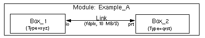
Figure 2.1 - Elements of topology for module called Example_A.
2.1 Box Attributes:
Each kind of object has attributes. Boxes have two attributes:- Instance-name - Name uniquely identifying each box in a diagram.
- Type - Specifies device-type or module-type that the box represents.
2.2 Link Attributes:
Links have six attributes:- Direction - fdplx, hdplx, smplx.
- Rate - Data transfer rate in MBytes/Second.
- Latency - Fixed overhead in mSeconds.
- QueueSize - Input/output buffer size in messages or -bytes.
- Route-Cost - Relative routing cost.
- PortNames - Port name on each end of the link.
The link transfer rate attribute specifies the number of data bytes that transfer across the link per mSecond, once the fixed overhead has been accounted for. The transfer rate is expressed in MBytes/Second. The fixed communication overhead specifies the time delay incurred by all message transfers regardless of message size. It is specified in mSeconds.
The transfer rate and latency attributes determine the time required to transfer a data message of given length according to the following link-model equation:
   		   MessageLength
     Ttransfer =  --------------- + FixedOverhead
   		   TransferRate
The link model takes into account any fixed overhead that may accrue such as from communications software driver routines, DMA setup, header generation/transfer, etc., that must occur before the application data begins transferring. The transfer rate is the rate that the data moves once it begins transferring. This rate is basically independent of the data length.
Direction:
The direction attribute is one of smplx, hdplx, or fdplx, depending on whether the links are simplex, half-duplex, or full-duplex. In simplex mode, messages may travel in only one direction, namely only from the first to second device to which the arrow points. In half-duplex mode, messages may travel in either direction, but only in one direction at a time. In full-duplex mode, messages may flow in both directions simultaneously, and the ports are treated as two separate simplex ports that run in opposite directions. Both hdplx and fdplx links are drawn with arrows on both ends. In other words, simplex links are uni-directional, while half-duplex and full-duplex links are two types of bi-directional links.
Queue-Size:
The queue size attribute specifies the maximum number messages or bytes which may be queued up on a port before further send operations are blocked. The queue size can be critical for processor synchronization and memory buffer space issues. The queue size must be an integer. Positive values specify the queue size in terms of the message count. Negative values specify the queue size in bytes (absolute value). The former is useful for modeling systems having a single message size or fixed buffer allocation. The latter is useful for systems having variable message sizes with dynamic buffer allocation.
Positive values must be greater than or equal to 1. A queue size of "1" indicates that a sending device will be blocked if tries to write a new message to a port on which the previous message has not yet been read by the receiving device. If blocked, operation will resume when the pending message is read. A queue length of "2" allows two messages to be enqueued before blocking, etc. If you never want blocking in your model, then use wild card "*" which indicates infinity.
Link-Cost:
The link-cost can be used to avoid using topologically shorter paths which may be slower or less desirable. The link-costs are intended to be used with the variable-cost routers.
The routing cost can help you control which paths the router will choose to get from place-to-place. The router considers the total cost to get from source to destination as the sum of the costs on each of the intermediate links. The default link cost is 1.0. A lower cost, such as 0.4, makes the link more attractive as a routing choice. A path containing two links each costing 0.4 appears shorter to the router than one link costing 1.0, (0.4 + 0.4 = 0.8, which is less than 1.0).
A higher routing cost makes a link less attractive. For example, a cost of 10.0 means that paths containing as many as nine cost=1.0 link-hops appear shorter to the router than the single cost=10.0 link.
For bi-directional links, both directions normally take the same cost. However, you can specify the cost independently by placing both costs in the attribute field separated by a comma and/or spaces. The first cost is the from-to cost. The second specifies the cost in the to-from direction. (The first port-name is considered the from side, while the second port-name is considered the to side.)
Port-Names:
Port name attributes can be any character string. All ports should be explicitly connected. Ports that are not connected to anything should be connected to DEV_NULL to avoid warning messages about unconnected ports during preprocessing. The default device DEV_NULL has two port types: NC and null. NC stands for not connected, and will give a runtime error if a device tries to write or read from such a port. null is essentially a bit bucket, and it will absorb anything written to it during the simulation. Reads will simply never return.
2.3 Hierarchy:
Topologies can be hierarchical. Hierarchy is expressed when a box instantiates a module which in turn is described by another diagram. Modules are instantiated at various levels of the hierarchy. The highest module in the hierarchy is called top_level. Boxes that do not represent modules are called, leaf-boxes, because they are the ends of hierarchical branches. Leaf-boxes instantiate device types which must have a behavioral definition and which contain no further decompositional structure.
By convention, leaf-boxes are drawn with thin lines, while boxes that represent modules
are drawn with thicker lines, as shown in figure 2.2.
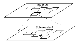
Figure 2.2 - Hierarchical topology diagrams.
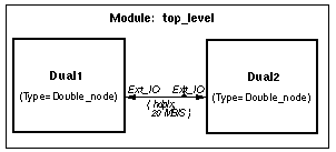
Figure 2.3 - Top-level topology.
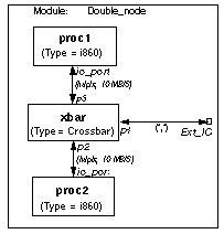
Figure 2.4 - Sub-module topology.
The structural hierarchy is a conceptual convenience. It is a way of grouping related
objects and hiding detail. At all times, the hierarchy can be equated to its flattened form
in which all modules are expanded onto a single-level diagram. Figure 2.5 shows the
equivalent flattened view of the hierarchical topology implied by figures 2.3 and 2.4.
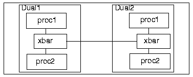
Figure 2.5 - Equivalent topology expanded to flattened hierarchy.
From within a module diagram, links that connect through the heirarchy are drawn to external port connections, which are depicted as small orange boxes.
2.4 Wild Card / Infinity "*" Attribute Values:
Often it is convenient to defer specifying some or all of the link attributes. For example, one case is when defining a general purpose module that may be instantiated in various systems with differing parameters. A second case is when the default link-delay mechanism is not wanted because the model will account for transfer delay in another way. For either case, use the "*" (asterisk) symbol instead of a literal value.The "*" serves as a wild-card or infinite speed attribute. In the first case above, consider a module with a link having a "*" attribute that connects to a link on another hierarchical module which has a finite literal value. The link attribute will then resolve to the finite value. It will not be considered a mismatch. In the second case above, any link attribute that does not resolve to a non-"*" value, will take on:
- an infinite value, if the attribute is transfer-rate or queue-size,
- 0.0, if the attribute is latency, and,
- fdplx, if the attribute is direction.
(Table of Contents.)3.0 Device Behavior Descriptions:
The device behavior describes the actions of each kind of device in a modeled system. A system usually contains several types of devices. There can be multiple instances of each type. CSIM provides means for describing a behavioral model for each type by providing mechanisms to:- Encapsulate C-language descriptions specific to each model type,
- Control variable scoping relative to each model instance,
- Manage the passage of simulated-time, and communicate between entities,
Figure 3.1 shows the basic structure of a behavioral model. Keywords are in all-caps, as
they must be. The model begins with the DEFINE_DEVICE_TYPE: keyword,
followed by the name of the type being defined. The names of the device's ports are then
listed in the PORT_LIST. Next, the variables that are local to each instance of the model
are declared using standard C variable declaration syntax. These are also called state-
variables or shared-variables because they can be accessed or shared by all the threads
within a given instance of the this model type. However, they are truly local to an entity
instance because CSIM ensures that each instance will get a unique set of the variables.
(See scoping level-2.)
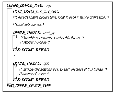
Figure 3.1 - Structure of behavioral model.
A thread definition begins with the keyword, DEFINE_THREAD: followed by an arbitrary thread name. The thread body is a standard C code block enclosed in brackets {}. As in any C code block, local variables can be defined at the beginning of the block. These variables will be local to each instance of the thread. Multiple instances of a given thread can be active within a given entity. Each will have a unique set of the local thread variables that are not accessible by other thread instances. (See scoping level-3.)
The local variable declarations within a thread are then followed by arbitrary standard C code. As with any C code, arbitrary expressions and control constructs, such as if, while, and for, can be written. Subroutines, print statements, input statements, and file operations can be called as well.
3.1 Variable Scoping Levels:
There are three distinct levels of variable scoping:- Global - Globally accessible to all entities and all threads.
- Shared - Shared by all threads within one entity. Local to each entity instance.
- Local - Local to each thread instance in each entity. (See Limitation.)
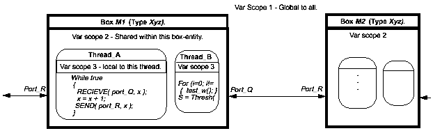
Figure 3.2 - Levels of variable scoping.
3.2 Standard Pre-defined Variables:
In addition to the user's variables, three standard predefined variables are accessible from all C-code. The standard predefined variables are:
The CSIM_TIME is a double floating-point value containing the current simulation time.
The same common value of CSIM_TIME accessed by all C-code in every model. Therefore CSIM_TIME is classed as a global scope-1 variable.
The MY_NAME variable is a character string containing the device's instance name. Its value will be entity specific. (All user C-code runs under threads from specific entity instances.) Therefore, MY_NAME is classed as a scope level-2 variable. The instance name will take on a hierarchical /xx/yy name based on where the device is instantiated within the topology.
MY_ID is a unique integer assigned to each device. These ID numbers start at zero and are contiguous.
The THREAD_VAR may be used to point to parameters that are specific (or unique) to the given thread instance. Therefore, THREAD_VAR is a scope level-3 variable.
3.3 Thread C-Code: : DELAY, SEND, RECEIVE, TRIGGER_THREAD
Each device description consists of a set of one or more C-language threads. Within the thread(s), the application algorithm is performed. From the C-code, the device can be made to send and receive messages/data to and from other processors in the modeled system. It can be made to initiate other threads or subroutines in parallel or sequentially. Time delay statements may be placed in the code to mimic processing delays, etc.Each device description must contain a thread called start_up. On simulation startup at time zero, each device begins execution from its start_up thread. Control can jump to other threads after the start_up thread is executed, or the whole program can exist as the start_up thread (with loops etc.).
There are four major routines which are used to manage the passage of
simulation time and communication with other devices. These are listed below:
The DELAY() function provides a way of mimicking a simulated time delay in your
code. The delay amount argument is a double floating-point value in simulation time
units; usually mseconds. After the specified time, the process will reawaken and
continue processing beyond the delay statement. Delay statements may be placed
anywhere in code threads or subroutines. The formal definition of the Delay function is:
void DELAY( double delay_amt ).
The TRIGGER_THREAD() function initiates execution of a code-thread after a specified time. It initiates parallel activities within the device, also known as forking or spawning. The trigger function is non-blocking and consumes zero simulation time. Multiple trigger commands can be made in a given thread routine without delaying the calling thread. The first argument must be a defined thread for the device. The second argument is the delay amount which is a double floating-point value and is in simulation time units. A value of zero causes the triggered thread to begin execution at the current simulation time. The third argument can be used as a parameter or a pointer to a unique set of variables which will be local to the triggered thread. It can be used simply as an integer identifying the thread when multiple instances of a thread are active within a given device. See guidance about passing user data for more information about type-casting. The thread_var for a thread can be accessed within the thread by the variable name: THREAD_VAR. The formal definition of TRIGGER_THREAD is:
void TRIGGER_THREAD( thread_name thread, double delay_amt, void *thread_var ).
The SEND() command causes a message to be sent out a given port to another device. The first argument specifies the port to use. The port name must be consistent with the port-names as defined in the topology. The second argument is the message pointer. Basically, the message pointer can be an integer message or it may be a pointer to any desired message data. See guidance about passing user data for more information about type-casting. The third argument is the message length. The message length value is used to determine the transfer time for the message. (It is divided by the link data-rate, as specified in the topology, and added to the fixed link overhead, to determine the simulation time needed to transfer the message across the link.) During the message transfer time, the link is declared in-use, and other messages would be blocked. The formal definition of the SEND function is:
void SEND( char *port, void *message_ptr, int length ).
The RECEIVE() command is the way of dequeuing a message from a queue. If there are no messages pending, the calling thread will sleep until a message is available. If there is a message, the message pointer will be returned into the second parameter, the amount of data received will be returned into the third parameter, and the message will be dequeued from the corresponding queue. (Note that the second and third parameters must be pointers to message data and integer respectively, since they will return the address of the message and an estimate of the length of data received respectively.) Note that the length estimate is not valid in the case where the incoming link transfer rate is set as infinite. See FAQ2-QA8 for more information about the calculation of the returned length estimate. The formal definition of the RECEIVE function is:
void RECEIVE( char *port, void *message, int *length_est ).
Related to the SEND/RECEIVE calls, are a set of routines for checking the status of a link, as well as the incoming and outgoing buffers.
- int CSIM_CHECK_IN_PORT_QUEUE( const char *port_name )
- int CSIM_CHECK_OUT_PORT_QUEUE( const char *port_name )
- int CSIM_CHECK_LINK_IN_STATUS( const char *port_name )
- int CSIM_CHECK_LINK_OUT_STATUS( const char *port_name )
The CHECK_OUT_PORT_QUEUE function checks the output queue of the named port of the current device. It returns the number of tokens in the queue. If there are none, then it returns zero.
The CSIM_CHECK_LINK_IN_STATUS and CSIM_CHECK_LINK_OUT_STATUS routines return information about any messages currently transferring across the link attached to the named port. They return zero if no items are presently transferring, and true (1) if an items is transferring. For half-duplex links, the in-and-out status is identical.
Comments can be placed anywhere. Comments can be made using the regular C language comment syntax, "/*" for begin comment, and "*/" for end comment.
3.4 Example Behavioral Description:
An example device type definition is described below. It is an illustrative but otherwise pointless routine that starts by sending a message out its port called port1. Then after a delay of 100 time units it initiates the gen thread which begins to periodically send messages out port2. Each time it does, the thread replaces itself by generating two instances of itself. The first of the two spawned threads begins execution while the original gen thread is still active, because the original is held up by a DELAY statement. Each instance of the gen thread dies away after executing its second trigger statement because that is the end of the thread code block. (There is no implicit loop at the end of a thread. Any looping must be explicit.) If allowed to continue indefinitely, the number of gen threads operating would grow geometrically. However, as an example this serves to illustrate several useful ideas.
        DEFINE_DEVICE_TYPE:     MC68030

           PORT_LIST( port1, port2 );

           /* Local Shared Variables */
           int message, counter;


           DEFINE_THREAD:  start_up
	     {
	       if (strcmp(MY_NAME,"Kingpin")==0)
		{
		 message = 1;
		 SEND( port1, message, 1.0);
		 TRIGGER_THREAD( gen, 100.0, THREAD_VAR );
		}
	     }
	   END_DEFINE_THREAD.


           DEFINE_THREAD:  gen
	     {
		counter = counter + 1;
		message = counter;
		SEND( port2, message, 1.0 );
		TRIGGER_THREAD( gen, 10.0, 0 );
		DELAY( (double)counter + 20.0 );
		TRIGGER_THREAD( gen, 100.5, 0 );
	     }
	   END_DEFINE_THREAD.

        END_DEFINE_DEVICE_TYPE.
Port-Types:
You can designate the type of connections that are allowed on specific ports by using the PORT_TYPE construct:
PORT_TYPE( {portname}: {type(s)} );
Example:
PORT_TYPE( port1: integer );The type names are arbitrary, but will be checked in the GUI when someone connects two boxes via a link. If a port-type was assigned on both sides, they must match. Otherwise the user will see a warning pop-up. You can allow multiple types of connections by listing them.
Example:
PORT_TYPE( port_out: floating_vector, integer, ctsrings );Ports with no types specified allow connections to other ports of any type. The PORT_TYPE construct can be used instead of the PORT_LIST. You do not need to list a given port in both methods. For example, if you assign types to all of a box's ports, you can just use the PORT_TYPE constructs:
        DEFINE_DEVICE_TYPE:     ControlBox
	  PORT_TYPE( port_in:    command_struct, data_record_coords );
	  PORT_TYPE( enable_sig: integer, cstrings );
	  PORT_TYPE( port_out:   floating_vector );
	  ...
3.5 Local Subroutines:
Subroutines that reference entity shared-variables as if they were global variables, without passing them through the argument list, must be defined locally within the device-type definition. Such subroutines are called local subroutines. Local subroutine definitions should be placed within the following keywords, which should be placed within the device-type definition after the shared-variable declarations, but before the thread definitions:
        /* Shared variable declarations.*/

        DEFINE_SUBROUTINE:

	  /* Place local subroutines here. */

        END_DEFINE_SUBROUTINE.


        /* Thread definitions. */
3.6 Global Definitions:
It is often convenient to declare some variables or subroutines globally to be sharable by all entity types and instances. This is scope level-1. See scoping-levels. Items which can be declared globally are:- Data structure definitions,
- Global variables, initial values,
- Global subroutines
- Macro definitions
        DEFINE_GLOBAL:
          /* Global variable declarations. */

          void scale_vector( x, y )
            {
              /* C-subroutine-code*/
            }
        END_DEFINE_GLOBAL.
There can be multiple DEFINE_GLOBAL sections among the CSIM source files. They
will all be combined by the pre-processor. Globally defined subroutines can be called
from any device behavior thread, and can access global variables and variables passed as
arguments. Examples of typical global variables include, file pointers for writing global
event history from any device, common mode setting variables, verbosity levels, etc..
3.7 Include Directive:
A special include directive called %include, works like the regular C-include, but is directed to the CSIM preprocessor itself. The regular #includes are not expanded by CSIM, but %include will be. This is especially useful in composing a system simulation consisting of separate topology and behavior component files. It can be used to configure specific architectures from various library files.3.8 CSIM_PRINTF and CSIM_ANNOUNCE:
Often when doing printfs to the screen from a device, it is helpful to first print the current simulation time and the name of the device from which the printf is coming. The CSIM_PRINTF and CSIM_ANNOUNCE functions provide convenient ways of doing this.
To use CSIM_ANNOUNCE, place a call to CSIM_ANNOUNCE ahead of your print
statement, as follows:
CSIM_ANNOUNCE(); printf("This is my message.\n");
An example screen output would appear as follows:
996.3475: /board1/cpu7: This is my message.
CSIM_PRINTF, is a macro that expands to the above expression. To use it, replace your normal printf( with:
	csim_printf(
as in:
	csim_printf("This is my message.\n");
The result is the same as above.
Note that CSIM_PRINTF is nothing more than a convenience macro that expands into two print statements.
3.9 RECEIVE_IR, RECEIVE_ALL_PORTS, and RECEIVE_ANY:
RECEIVE_IRSometimes it is desired to model a device that responds when data is first beginning to arrive, even though the data will be streaming in for a while before the message is complete. Such an example is a worm-hole crossbar, which begins transmitting data as the data comes in. Normally, a RECEIVE call does not return until all the data has arrived. To help model the other case, a modified version of RECEIVE, called RECEIVE_IR, is available. RECEIVE_IR stands for RECEIVE with Immediate Return. The formal definition is:
void RECEIVE_IR( char *port_name, void *message, int *length )
RECEIVE_IR behaves just like RECEIVE, except that it returns immediately when a message is sent after the overhead delay has occurred, instead of only after the message has completely arrived (td = overhead + length / rate). Yet the link will remain busy for the full message duration. Another major difference is that RECEIVE_IR does NOT dequeue the message. Therefore, RECEIVE_IR must always be used with a regular RECEIVE which will dequeue the message once it is complete. This can be relegated to a forked-off RECEIVE thread if desired.
One caution: since RECEIVE_IR does not dequeue anything, it will always return the next message to be received, no matter how many times it is called before an actual RECEIVE is made. This can be useful. For instance any number of RECEIVE_IRs can be pending and triggered off the same incoming message. Also, remember that RECEIVE_IR does not only return currently incoming messages. It returns the first message on the receive queue, even when there is not a message coming-in, as long as there is a message pending on the received queue (already came-in but not dequeued).
RECEIVE_ALL_PORTS
The RECEIVE_ALL_PORTS function is like the RECEIVE function, except it looks at all
the ports a device, instead of just one. It returns on the
first of the port's to receive a message. It is useful for receiving the first
arriving data from all of the ports. An alternative would be to
trigger a separate thread, each with a RECEIVE, for each port.
However, RECEIVE_ALL is much more efficient and convenient, being that it
uses only one thread, and you do not need to specify what the port-names are. The formal prototype is:
int RECEIVE_ALL_PORTS( void *message, *length )
RECEIVE_ALL_PORTS returns an integer indicating the port-number on which data was received.
RECEIVE_ANY
The RECEIVE_ANY function is like the RECEIVE_ALL_PORTS function, except it accepts a list of
port-names. It returns on the
first of these port's to receive a message, dequeuing the
pending receive from the other ports. It is useful for receiving the first
arriving data from any of a subset of the available ports. An alternative would be to
trigger a separate thread, each with a RECEIVE, for each of several ports.
However, RECEIVE_ANY is efficient and more convenient, being that it
uses only one thread. The formal prototype is:
int RECEIVE_ANY( char *(*port_list), void *message, *length )The port_list must be an array of character-string port names. The final element of the array must be zero.
Example:
	char *port_name_list[n+1];
	port_name_list[n] = 0;
Where n is the number of port names in the list.
RECEIVE_ANY returns an integer indicating the index of the port-name in the port-list causing the return. I.E. The port on which data was received.
In every other respect, RECEIVE_ALL_PORTS and RECEIVE_ANY operate like the regular RECEIVE function relative to blocking, dequeuing, and returning the message and its length. RECEIVE_ALL_PORTS r and RECEIVE_ANY are analogous to the select function of unix shell. See also Listing Ports for an automatic way of creating the port-list array.
RECEIVE_IR_ANY
The RECEIVE_IR_ANY function is a combination of the RECEIVE_ANY and RECEIVE_IR
functions described above. It accepts a list of port-names and returns
when the first of these has begun receiving a message. Like RECEIVE_IR,
it does not wait for the message transfer to complete; nor does it dequeue
the message. See above.
3.10 Preempting or Re-Scheduling Future Events: PREEMPT_INCOMING, PREEMPT_OUTGOING, CSIM_PREEMPT_EVENT, CSIM_RESCHEDULE_EVENT
The activation or resumption of a thread is often referred to as an event. Events scheduled to occur in the future can be preempted, or re-scheduled, before they occur. Examples include, (A) the scheduled completion of a message transfer across a link, or (B) the activation of a thread scheduled by TRIGGER_THREAD with a future time.A. Preempting Incoming or Outgoing Port Transfers:
The PREEMPT_INCOMING and PREEMPT_OUTGOING functions are a way of preempting message transfers while they are in progress. The preempt functions take one argument, the port name on which the transfer is to be preempted. If there was a RECEIVE waiting for the transferring message to complete, the RECEIVE will return immediately, and it will return in its length field the number of data units that transferred up to the preemption. If there are pending sends, they begin immediately after preemption of the current message. If there is no message being transferred, then nothing happens.
To distinguish direction, the preempt call is one of either:
PREEMPT_INCOMING(), or PREEMPT_OUTGOING().
B. Preempting Threads Triggered to Begin in the Future:
Threads that were triggered to begin execution in the future, after a time delay, can be preempted
before they occur, by calling the CSIM_PREEMPT_EVENT function with the REMOVE_EVENT method. Likewise,
the delayed execution of a thread can be preempted with the FORCE_EVENT_NOW method.
The function is defined as:
CSIM_PREEMPT_EVENT( ThreadID, Method );The Method value can be either REMOVE_EVENT or FORCE_EVENT_NOW. The thread-ID can be obtained for a future scheduled thread, as the return value from the TRIGGER_THREAD call, or for the current thread by the CSIM_GET_THREAD_ID() function which is defined as:
int CSIM_GET_THREAD_ID()Example usage:
	int threadID;

	threadID = TRIGGER_THREAD( xyz, 200.0, 0 );
	DELAY( 10.0 );
	if (nolongerneeded)
	 CSIM_PREEMPT_EVENT( threadID, REMOVE_EVENT );
The related function:
int CSIM_EVENT_CHECK( int threadID )can be used to check if a given thread-ID still exists, or if a scheduled event is still pending. It returns 1 if it does. Otherwise it returns 0.
A more efficient variant of CSIM_PREEMPT_EVENT, called CSIM_PREEMPT_EVENT_AT, can be used when the time of the event is known. The function is defined as:
CSIM_PREEMPT_EVENT_AT( int ThreadID, int Method, double event_time );The first two arguments are the same as above. The event_time is the time for which the event to be removed, was scheduled for.
C. Rescheduling Thread-Events to Other Future Times:
The CSIM_RESCHEDULE_EVENT function is
similar to CSIM_PREEMPT_EVENT_AT above, but instead of removing the event, it
changes the time of the event. Note that only pending future events can be rescheduled.
And they can only be rescheduled to future (or current) times. Unlike most of the other
event-scheduling functions, such as as DELAY, TRIGGER_THREAD, or CALL_THREAD,
which are time-relative, the times in this function must be absolute.
For example, to reschedule an event to occur 5.0 units from the present time, use CSIM_TIME+5.0.
The function is defined as:
CSIM_RESCHEDULE_EVENT( int ThreadID, double scheduled_absolute_time, double new_absolute_time );It reschedules the previously scheduled pending event to a new absolute time.
3.11 Animation Highlighting:
The simulator can be run from either a text-only command-line interface, or from a graphical control window. The latter provides the capability to visually animate your models. It allows navigation over your topology diagrams while the simulation runs. The following highlight functions and the related annotate functions fulfill the purpose of animating the diagrams with significant events during the simulation.The highlight_box function causes the box which contains the calling code to change to a specified color. The highlight_link function causes the specified link to change color. These functions can be used to provide meaningful visualization of the processes you are modeling. They are active under the user-animation mode of the graphical simulation control window. They are ignored by the text-only command-line version of the simulator. The visualization functions are formally defined as:
	highlight_box(  int color );
and
	highlight_link( char *port_name, int color );
The following variants of highlight_link are useful for animating directional transfers on bi-directional links:
	highlight_inlink( char *port_name, int color );
and
	highlight_outlink( char *port_name, int color );
The in and out indicate the direction of the transfer to be animated. State information is maintained so that the proper color is displayed when transfers are initiated or terminated from either end.
You can put these anywhere in your models to indicate significant events. They are relative to the entity of the thread that calls the highlighting function.
Example usage:
        highlight_box( Red );
        DELAY( 10.0 );
        highlight_box(  0 );
        highlight_link( "p3", Green );
        DELAY( 10.0 );
        highlight_link( "p3", 0 );
The following colors are macro-definitions that are valid in every simulation:
         Black    0         Green    9
         Fuchsia  1         Violet  10
         Blue     2         Orange  11
         Cyan     3         Gold    12
         Gray     7         Pink    13
         Red      8         White   15
You can use these colors or their numbers directly. The color Black or 0 returns the
object to its original default color. By default, 232 colors are predefined.
(click to see the color palette.)
In addition to the standard 16 colors, you can specify an arbitrary Red, Green, Blue
color value by using the color_lookup( r, g, b ) function. Specify
each component in the range 0 - 255, where 0 is dark, and 255 is bright.
Example:
highlight_box( color_lookup( 200, 143, 30 ) );
For animating wireless networks, see Radio Animations.
3.12 Annotation Animation:
The annotate function can be used to write textual information on the graphical display near boxes during simulations. The formal definition is:Annotate( char *strng, int color, float xoffset, float yoffset);
It is very much like the highlight_box and highlight_link functions described in 3.11,
except that it writes text near the entity that calls it. A suggestion is to use this for
debugging. You can make the annotation be conditional on a verbosity value. You
could use it to show internal states of all devices during execution. Below is an example
usage:
Annotate( "Connecting Ports", Green, 0.0, -0.5 );
By default, if the xoffset and yoffset are 0.0, it will put the text string in the center of the box that corresponds to the entity that called it. The xy-offset values will offset the position of the text relative to the center of the box. (Units are in inches. Initial diagrams are roughly 8.5 inches high by 11 inches wide. So it helps to think in terms of a sheet of paper and a ruler.) Some trial and error usually helps.
Positive y-offsets are down, positive x-offsets are to the right. The above example writes
the text above the box because the y-offset was -0.5. It is ok to put the text inside the
boxes. If you do, then it helps if you turn-off the box instance-names and type-names
(under the View menu) when running the simulation. Below is another example:
       {
        char mesg_strng[50];

        sprintf( mesg_strng, "Connection: %d %d", state1, state2 );
        Annotate( mesg_strng, Green, 0.0, 0.0 );
       }
You could use this to view changing state information or to note specific events or
unusual events. It can be more visual than the standard printouts, because it is placed
with the respective boxes in the diagram.
The available colors are the same as stated in 3.11. To erase a previously written annotation. Call Annotate with the previous text string, but with the color Black. The size and position of a given box can be determined by MY_POSITION, defined as:
void MY_POSITION( char *obj_name, float *pos_x, float *pos_y, float *xsz, float *ysz )To determine a box's size to adjust the annotation offsets to display at the box origin, you could use for example:
        float x, y, boxwidth, boxheight;

        MY_POSITION( MY_NAME, &x, &y, &boxwidth, &boxheight );
        Annotate( "Message", Green, -0.5 * boxwidth, -0.5 * boxheight );
3.13 Synchrons: WAIT, RESUME, RESUME_WITH_PARAM, WAIT_WITH_TIMEOUT, SCHEDULE_RESUME_WITH_PARAM
The WAIT and RESUME functions are methods for controlling the execution of threads without the need for hardwired links or SEND/RECEIVES. When WAIT is called from a thread, the thread goes asleep until awoken by a RESUME call from another thread. A RESUME is directed to a specific waiting thread (or group) by means of a special identification variable, called a SYNCHRON.The WAIT_WITH_TIMEOUT function is a combination of the DELAY function described in section 3.3, and the WAIT function described here. It blocks its calling thread until the first of either its synchron is resumed or its time-delay has expired. The following method is suggested for determining whether awoken by time-out or explicit resume: (1) Resume the synchron only by RESUME_WITH_PARAM and pass a non-zero parameter or address; (2) On awakening from WAIT_WITH_TIMEOUT, check the value returned. If zero, then awoke due to time-out. If non-zero, then awoke due to explicit resume.
The RESUME_WITH_PARAM function enables the resumer to pass a parameter or pointer to any waiting thread(s). Any WAIT calls so resumed, will return the parameter. This is sometimes helpful to distinguish who out of many, resumed a given thread.
The SCHEDULE_RESUME_WITH_PARAM function enables you to schedule a resume to occur for a synchron at a future time. The value returned by the eventually resumed WAIT will be the value of the user-parameter when SCHEDULE_RESUME_WITH_PARAM was called. One use is in cases where the thread which calls SCHEDULE_RESUME_WITH_PARAM, is to die or goes off to do other things, before the resume is to occur. In some cases, it can be used as an efficient alternative to TRIGGER_THREAD, for scheduling delayed executions. (Thread creation/destruction can be more costly than waiting on a synchron from a persistent thread.)
The formal definition of the WAIT, RESUME, RESUME_WITH_PARAM,
WAIT_WITH_TIMEOUT, SCHEDULE_RESUME_WITH_PARAM, and related functions are:
  void *WAIT( SYNCHRON **x, int flavor );
  void RESUME( SYNCHRON **x, int flavor );
  void RESUME_WITH_PARAM( SYNCHRON **x, int flavor, void *user_parameter );
  void *WAIT_WITH_TIMEOUT( SYNCHRON **x, int flavor, double time_delay );
  void SCHEDULE_RESUME_WITH_PARAM( double time_delay, SYNCHRON **x, int flavor, void *user_parameter );
The SYNCHRON must be initialized to zero prior to usage; normally at the start of a simulation.
This can be accomplished with the NEW_SYNCHRON() function.
An example usage is:
        DEFINE_DEVICE_TYPE: procA
          SYNCHRON *synchpt_A;

           DEFINE_THREAD: start_up
            {
	     synchpt_A = NEW_SYNCHRON();
             TRIGGER_THREAD( procB, 0.0, 0 );
             DELAY( 100.0 );
             RESUME( &synchpt_A, NONQUEUABLE );   /* NOTE the & */
            }
           END_DEFINE_THREAD.


           DEFINE_THREAD: procB
            {
             WAIT( &synchpt_A, QUEUABLE );      /* NOTE the & */
             csim_printf("Proc_B awake\n");
            }
           END_DEFINE_THREAD.

        END_DEFINE_DEVICE_TYPE.
In this example, a local shared variable called synchpt_A is declared. It will be a
synchron variable. This is how you would specify what to wait-on or what to resume.
At time=0.0, the start_up thread spawns the procB thread and then delays for 100.0. The
procB thread goes into a WAIT on the synchpt_A synchron. At time 100.0, the start_up
thread does a RESUME on the synchpt_A synchron, which wakes up the procB thread.
There are two versions of the WAIT and RESUME functions:
(The type SYNCHRON is a predefined data type.)
Explanation:
WAIT( &synchr_x, QUEUABLE )If several threads are waiting on the synchron, then upon a RESUME, only one waiting thread will awaken. (One RESUME awakens one waiting thread.)
WAIT( &synchr_x, NONQUEUABLE )If several threads are waiting on the given synchron, then upon a RESUME, all waiting threads will awaken at once. (One RESUME awakens all threads waiting on the synchron.)
RESUME( &synchr_x, QUEUABLE )If NO threads are waiting on the given synchron, then the fact that a RESUME occurred will be queued. When the next WAIT occurs on this synchron, it will dequeue the RESUME and continue immediately without going into a wait. (RESUMES are remembered if nothing is waiting.)
RESUME( &synchr_x, NONQUEUABLE )If NO threads are waiting on the given synchron, then the RESUME will not be stored (or queued). When the next WAIT occurs on the synchron, it will sleep until a RESUME is issued. (RESUMEs must occur after WAITS to have an effect.)
CHECK_SYNCHRON returns the number of threads waiting on a given SYNCHRON. In any case, it will not block. If nothing is pending on the SYNCHRON, then it returns zero. If no threads are waiting, but RESUMEs are queued, then it returns the number of RESUMEs as a negative number.
The formal definition of this function is:
int CHECK_SYNCHRON( SYNCHRON *x );
Here is an example that uses CHECK_SYNCHRON:
    DEFINE_DEVICE_TYPE:  test_device
     SYNCHRON *A;

     DEFINE_THREAD: start_up
      {
       A = NEW_SYNCHRON();
       TRIGGER_THREAD( procB, 0.0, 0 );
       csim_printf("%d threads are waiting.\n", CHECK_SYNCHRON( A ) );
       DELAY( 100.0 );
       csim_printf("%d threads are waiting.\n", CHECK_SYNCHRON( A ) );
       RESUME( &A, NONQUEUABLE );
       csim_printf("%d threads are waiting.\n", CHECK_SYNCHRON( A ) );
      }
     END_DEFINE_THREAD.


     DEFINE_THREAD: procB
      {
       csim_printf("This is from thread Proc_B\n");
       WAIT( &A, QUEUABLE );
       csim_printf("Thread Proc_B is now awake\n");
      }
     END_DEFINE_THREAD.

    END_DEFINE_DEVICE_TYPE.
WAIT can optionally return a parameter passed by the resumer.
For an example, see resumewparam-example.
(Or right-click to download resumewparam.sim.)
The CLEAR_SYNCHRON() function can be used to reset a synchron to its initial state. It will clear any pending resumes or waits from the given SYNCHRON.
The formal definition of this function is:
void CLEAR_SYNCHRON( SYNCHRON *synchr_ptr );
3.14 Halt and CSIM_HALT_POPUP:
The halt function can be placed anywhere within user-code. It can be used to stop simulations. When encountered during a simulation, it causes the simulation to pause, and control returns to the control panel or simulation prompt. Just as when the simulation pauses due to a breakpoint, step, crawl, or other reason, the user can choose to resume the simulation, quit, or examine other options.
Here is an example that uses halt:
	if (unexpected_event)
	  halt();
If the user continues execution, the simulation will resume executing from directly after
the halt function.
The halt function is often useful for:
- Inserting conditional breakpoints into a simulation.
- Breaking in (or on) specific subroutines or lines of code.
- Calling attention when assertions have been violated.
- Stepping by significant events instead of time amounts.
- Detecting and forcing a simulation end-point.
- Many other reasons, as needed.
When running graphical simulations, it is often helpful for models to popup a message window when something extraordinary happens. This brings attention to the user. A model can popup a message window by calling:
CSIM_HALT_POPUP( char *message )With the message as the argument.
A popup window will appear with your message in it. The popup has a dismiss button on it.
Example:
CSIM_HALT_POPUP( "Special event occurred." );Or,
Copy your message into a string ...
char mymessage[60];
sprintf(mymessage,"%s Over temperature by %f degrees", MY_NAME, x);
CSIM_HALT_POPUP( mymessage );
3.15 Conditional Model Inclusion (%ifdef, %ifndef, %define):
Often some of your model files, which were developed separately, may contain repeated definitions if used together in the same simulation. In standard C, this kind of situation is remedied with the #ifdef, #ifndef, #endif, and #define constructs. These constructs effectively sensitize or desensitize the C compiler's preprocessor to sections of your code.However, in CSIM the C compiler runs after the CSIM-preprocessor, so all the #ifdef, ... etc., sections are still visible, which may cause the preprocessor to see multiple definitions.
Therefore, the CSIM-preprocessor has been made sensitive to the following
useful keywords:
	%define
	%ifdef
	%ifndef
	%endif
These can be used to conditionally sensitize the CSIM-preprocessor to
certain sections of your model code. They can be used as follows:
	/* Wrap potentially repeated sections of your model code in sections like this. */
	%ifndef someuniquename
        %define someuniquename
           { Contents of your model, definitions, etc.. }
	%endif
Desensitized sections of your code will not be passed to the C compiler and
are ignored by CSIM's preprocessor as well.
3.16 CSIM_EXIT_THREAD()
Causes the executing thread to end. Returns control to other threads within a simulation. Can be called from anywhere, such as inside a loop or from a subroutine. All the thread's resources (data structures) will be removed. This is useful when a thread is no-longer needed. It helps reduce the number of active threads, which improves efficiency.The CSIM_EXIT_THREAD() call is equivalent to returning from a thread (I.E. falling through the bottom of a DEFINE_THREAD block). Therefore, it is unnecessary under normal circumstances. However, CSIM_EXIT_THREAD() is useful when the need to end a thread is detected in a deeply nested block.
3.17 Model Attributes
A very important and powerful modeling construct is the concept of model attributes, along with their related functions. Attributes may be set to numeric (integer or floating-point) values, character strings (such as names or enumerations), or even complex expressions containing other attributes or common math functions. They can act as macros or variables. Macros enable deferred evaluation and are interpreted during simulation, while variables offer immediate evaluation when set.
Attributes have two parts: a name, and a value. Each attribute is a name - value pair.
The name consists of a single word, while the value can be an expression.
Examples:
pressure = 14.7
degrees_C = (degrees_F - 32.0) / 1.8
Speed = Fast
Attributes, or parameters, can be set to values at various levels of a model's diagram hierarchy. When they are set at the top level, they are often called global simulation parameters, global macros, or simulation variables. When an attribute is set at particular diagram or module level, it is sometimes referred to as a graph variable. Attributes can also be set on individual box instances, where they are referred to as instance attributes. CSIM provides downward inheritance. Models inherit all attributes defined above them, but more local definitions override higher ones. Attributes can take default values, if not otherwise defined at a higher level.
Regardless of where an attribute is set, or what it is called, they all exist in the same name-space, are accessible by the models, and will inter-relate. Models may access attributes from their internal behavioral code. Attributes can be set, viewed, edited, or changed from the GUI, as well as by other tools, such as the Iterator without recompiling simulations. They can be used to quickly change modeling parameters, and/or to set aspects of individual entity behaviors.
More information about model attributes and their access functions, can be found in Instance Attributes.
3.18 Model Aliases
Often you may have a box behavior that is common among several boxes, but you want to differentiate the boxes in some way, such as by distinct meaningful type-names, different default icons or default attributes.Model aliasing allows a given behavior description to be referenced by multiple different model-type names, without copying all the code, as has been previously required.
For example, suppose you have two conceptually different kinds of network components, which actually have identical behavioral models underneath. You want to provide users the ability to call them different kinds of objects, but you do not want to maintain copies of otherwise identical device models.
You can do this be adding lines like the following to your model:
<alias_model alias="cisco5050" model="generic_router" />Then just define the "generic_router" model once. You can then instantiate models of types "cisco5050" and "NetGear600", which will simply use the generic_router model, although possibly with differentiating attributes and default icons provided by empty DEFINE_DEVICE: shells.
<alias_model alias="NetGear600" model="generic_router" />
(Table of Contents.)4.0 Simulator Usage:
The sections below describe how to build and run simulations.4.1 Building Simulations:
To build a CSIM simulation, first prepare the source file(s) describing the system you wish to simulate, as described in sections 2 and 3.- The system topology, and
- The device-type behavior descriptions.
csim arch.simThe CSIM preprocessor will then attempt to process your input files. If CSIM is successful, it will produce a compilable output file called, out.c. "out.c" is a processed text file of your original input file(s) along with the injected simulation kernel. If no preprocessing errors where detected, CSIM will attempt to compile this file using the C-compiler. If the compilation is successful, it will produce an executable called sim.exe. You can then invoke the simulation by selecting Run Simulation under the Tools menu of the GUI, or from the command-line by running the executable. For example:
sim.exe
[ Along with sim.exe, another file called top_tab.dat is also produced. It is accessed by sim.exe at simulation-startup. By default, it exists in the same directory that the simulation is built and run from. Therefore it is usually transparent to users. However, if you wish to run a simulation from a directory other than where where it was built, then set the environment variable CSIM_TOPTAB to point to the directory where it was built. ]If any problems are detected when building the simulation, diagnostic messages will appear within your text window. It is recommended to scan this window for the results of the build.
By default, CSIM builds the graphical version of the simulator. However, you have the
option to build the textual version by selecting Tools / Modify Commands / Build Textual Sim
from the GUI. Or from the command-line, by adding -nongraphical to the build
command.
Example:
csim -nongraphical my_models.sim
See Textual-Simulator for more information.
Build Verbosity:
When pre-processing your simulation models with CSIM, you can set the verbosity with which it prints diagnostic messages to the screen using the command line option -verbose x, where x is an integer indicating the verbosity level. For instance:csim my_models.sim -verbose 2
The verbosity levels presently span from 0 to 501, where 0 is the minimum, and 1, 2, 3, 4, ... provide progressively more detailed information. 0 is the default. The higher the verbosity level, the more information is printed to the screen during pre- processing. The higher levels are helpful when there are problems, since they give a closer indication as to where the problem is. Each higher level includes the lower level printouts.
Summary of Verbosity levels:
	 0 - Default, minimal output.
	 1 - Leaves intermediate files.
	 2 - Shows major intermediate processing steps.
	     Shows variable and macro definitions.
	 3 - Shows variable/macro substitutions intermediate steps.
	 4 - Shows more detailed build steps.  Additional checking reports.
	 6 - Messages about graph flattening, connecting links.
	 7 - Detailed summaries of links in processed graphs.
	10 - Port list parsing checks.
	11 - Attribute expansion printouts.
	21 - Summaries of links in intermediate flattening steps.
	41 - Arc data lists.
	51 - Show macro expansions. List detailed geometry info.
	101 - Variables listings.
	501 - Attributes listings.
See appendix H for more command-line options.
4.2 Running Simulations:
The simulator can be run from either:- the Graphical Control Window - Provides convenient push-buttons and menus for controlling the simulation. It also provides visual animation of your models with ability to navigate through your topology diagrams (or flatten them) while the simulation runs.
- a Text-only Command-Line Interface - Useful for running simulations from batch scripts, command-files, interactive programs, non-graphical terminals, or anyone preferring a conventional monitor/debugger type interface.
By default, the CSIM builds the graphical version. However, you can build the
textual version by selecting Tools / Modify Commands / Build Textual Sim
from the GUI. Or from the command-line, by adding -nongraphical to the build
command.
Example:
csim -nongraphical my_models.sim
In either case,
the respective simulator interface will then come up when sim.exe is invoked.
You will find that the same corresponding functions are available in either graphical or textual interfaces. The graphical simulator control panel contains buttons and menus corresponding to the commands available from the textual simulator interface. Additionally, the graphical version contains many features for animating simulation runs. More detailed description on using each of the interfaces is provide in sections Graphical-Sim and Textual-Sim below.
Breakpoints on Time:
Breakpoints at specific times can be set by selecting the Breakpoints button, and specifying a time for the breakpoint to occur. Hitting the Run button will cause the simulator to run up to the next breakpoint and stop. The simulation can be resumed by hitting the Run button again. Commonly, several breakpoints can be entered prior to starting the simulation run. New breakpoints can be added at any time.
Breakpoints on Model Source-Code Lines:
Breakpoints can be set to occur when specific subroutines, or sections of code are executed, by placing a halt(); at the specific location in the model source-code. The simulator will stop when it hits the halt(); instruction. The simulation can be resumed by hitting the Run button.
Conditional Breakpoints:
Conditional breakpoints of arbitrary complexity can be set by placing their conditions either in specific sections of particular models, or based on global parameters and placed in the common monitor block. In either case, the conditional evaluation should print a brief message describing or identifying the breakpoint and then branch to a halt() instruction.The simulator will stop when it hits the halt(); instruction. The simulation can be resumed by hitting the Run button.
4.3 Graphical Simulator
The graphical simulator control-panel is similar to the GUI-Diagram-Editor, except that many of the buttons specific to editing are replaced with buttons appropriate for controlling simulations. You can navigate your diagrams just as in the GUI-Diagram-Editor.When you invoke the graphical simulator, you will see buttons for controlling simulation execution and navigating on the left side of the control panel. Along the top panel, you will see pull-down menus for setting various simulation options. To the right of the top menu bar, you will see the simulation-time indicator and status indicator. In the center is your simulated architecture diagram.
The buttons for controlling simulation execution on the left side of the control panel include:
- Run/Continue - Clicking this button will cause the simulator to run until stopped by: a breakpoint, hitting the Stop button, a halt instruction within a model, or the end of the simulation when there are no more events. If stopped, the simulation can be resumed by hitting this button.
- Step - Clicking this button will cause the simulator to run until the next step-amount of simulated time passes. By default, the step-amount is initially set to 1.0 uSeconds. So hitting the Step button resumes the simulation until 1-uS of simulated time elapses, then it stops. You can change the step-amount to another quantity by clicking on the * button next to the Step button. The Step button is convenient for manually controlling the rate of simulation execution, by repeatedly hitting the Step button at the desired rate.
- Crawl - Run simulator for one event, then stop. The number of events to run, or crawl_amount, before stopping can be set by clicking on the * button next to the Crawl button. Crawl will always stop at a time boundary. For example, if the crawl_amount were set to 10000 events, but only four (4) events occurred for the current time, the simulation will stop. It can be resumed by hitting Run, Step, or Crawl. This is a convenient way to manually step by time increments.
- Stop - Stop simulator at any time. It can be resumed by hitting Run, Step, or Crawl.
- Breakpoints - Set breakpoints.
All functions for running, stepping, and stopping simulations, etc., are the same as for the textual simulator, except that they are invoked with buttons, or pull-down menu selections. See 4.4 Textual-Sim below for description of the available options.
Further down the left side of the control panel are the buttons for navigating diagrams. These are the same as in the GUI editor.
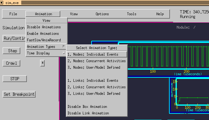
One of the primary options to set when running a simulation is the animation mode. There are several levels of animation control. The box and link animations can be controlled individually.
- All Animations On/Off (Enable/Disable_ - Simulations run quickest when animations are turned-off. Off overrides (but remembers) all selections below.
- Box Animations
- On/Off - Enable/Disable
- 1. Individual Events - Blink box where event occurs during each individual event.
- 2. Concurrent Activities - Light all boxes having events that occur concurrently at current time. (Keep them lit until time advances.)
- 3. User/Model Defined - Display only user animations - Explicit calls to the highlight_box function at specific places in the user's model-code.
- Link Animations
- On/Off - Enable/Disable
- 1. Individual Events - Blink link where SEND event occurs during each individual SEND event.
- 2. Concurrent Activities - Light all links having ongoing data transfers (concurrent display). (Keep them lit until respective data-transfer ends.)
- 3. User/Model Defined - Display only user animations - Explicit calls to the highlight_link function at specific places in the user's model-code.
- Time Indicator
- Update always.
- Update within specified time amount.
- Update every 10, 100, or 1000 time-advances.
- Do not update.
Updates to the screen-display can add significant overhead to simulation runs. Screen updates include animations and updating the time-indicator. However, sometimes the animated visualizations are very valuable. For example: while debugging, or for demonstrating or visualizing a proposed design's operation. When not needed, turning-off some or all of the animations, and reducing the updates of the time-indicator, enables simulations to proceed with virtually no overhead.
When interested in model behavior that occurs well into a simulation run, it is convenient to first turn the animations off. Run (quickly) up to a specific breakpoint of interest, and then turn the animations back-on there.
The state of box-animations is recorded, even when not animating. So you will see the current system state immediately when you turn the animations on, or when you switch animation modes, navigate, or re-size the window.
The state of link-animations is not recorded when not animating for efficiency reasons. Therefore, you will not immediately see the current link animation status when initially turned back-on. However, as the simulation continues, the link-animations will reach their proper states. In such cases, you may wish to turn the link-animations on at some time prior to the interval of interest. Once animating, all animation modes for the links are recorded, so you will instantly see the current valid link animation states even when you change the link animation mode, navigate, re-size, or re-draw the screen.
The animation modes are set by the Animation Menu which is the second item on the the top tool-bar. It is a two-level menu. Figure 4.3.2 shows how the animation menu of the simulation control panel cascades when selected.
See Graphical Simulation Control Panel for more information about the menus.
4.4 Textual Command-Line Simulator
The textual version of the simulator is especially useful for script-driven batch simulation runs, when no one is available to press the run button. It is also useful when no graphical output is needed.
You can build the textual version of the simulator from the GUI by selecting
Tools / Modify Commands / Build Textual Sim. Or from the command-line,
by adding -nongraphical to the build command.
Example:
csim -nongraphical my_models.sim
You can then invoke the simulation as normally from the GUI, or from the command-line
by typing sim.exe . The simulation will appear in your text window.
When the simulation begins, you will see the simulation prompt. At this prompt, you
can type h at any time for help. It is usually useful to set up the simulation displays
and breakpoints at this time. You can execute your simulation by stepping, or
running (s, or r). The step amount can be defined arbitrarily, but is defaulted to 1.0
time units.
Help Menu:

        v = verbosity settings
        r = run          - (run or resume)
        s = step         - (step by step amount time (s or step xx))
        c = crawl        - (step by a delta cycle (within time))
        b = break-points - (set break-points)
        show_links       - (show status of all links)
        fshow_links      - (dump links status snap-shot to a file)
        examine_link     - (examine status and queue of specific link)
        stats            - (Send link utilization statistics to file.)
        sim_status  - (Tells exactly what is about be executed, device, event, delta-cycle, etc..)
        show_active_links - (show just the active links)
        show_event_queue  - (show the current event queue)
        fshow_event_queue - (dumpt the current event queue listing to a file)
	rank_events	  - (show which boxes are generating the most events)
        list_devices -  (show a list of all the devices names in the simulated system)
        list_variables - (show a list of the local variables contained by a device and their
                                      current values)
        time            - (print the current simulation time)
        q = exit
You can step through the execution of your simulation by an arbitrary time amount,
know as step_amount, by simply typing s. When you do, the simulation will run for
however many time units are specified by the step_amount. By default, the step_amount
is initially set to 1.0 at simulation startup. So typing s will advance the simulation by one
time unit. You can specify the step amount by typing step xx, where xx is an arbitrary
floating-point step amount.
    Example:

         sim>  s
                (step amount = 1.0, stepping by 1.0)

      or

         sim>  step 0.25
                (step amount = 0.25, stepping by 0.25)
         sim>  s
                (step amount = 0.25, stepping by 0.25)
Similarly, the crawl command can be used to step by a single event by simply typing c.
Or you can step to a specific delta-cycle (within the current time instant) by typing
crawl xx, where xx is the delta-cycle number. Note that each event processed
corresponds to one delta-cycle. The delta-cycle number is an integer.
The sim_status command tells what device is being serviced, what event is being processed, and what delta cycle the simulator was on within the current time instant. It is especially helpful upon hitting a fatal error, since it can show you exactly what section of code was being executed at the time of the failure.
For non-interactive simulations, it is often useful to direct commands from a script file,
as in:
sim.exe < script.com > logfile &
.
Link Statistics:
During a simulation run, the CSIM kernel maintains statistics on each link in the form of
percent utilization and peak queue-lengths. You can take a snap-shot of this information
any time during the simulation, by simply typing stat at the CSIM prompt. CSIM will
then write the link statistics to a file called, link_stats.dat.
Event-Queue Statistics:
During a simulation run, you can see which boxes have the most
pending events, with the rank_events command. This is often useful for
optimizing simulations, and for determining which boxes may be generating an
inordinate amount of pending events. An example listing appears below:
   Sim>  rank_events

	Top 10 Boxes by Pending Events:
	(#Events   (By %)      Box)
	     1141   (56.4%)     /3000/9993100/9993200/3260/3265
	      584   (28.9%)     /5000/9995200/5219
	       97   ( 4.8%)     /14000/14300/14306
	       61   ( 3.0%)     /6000/6300/6900/6902
	       11   ( 0.5%)     /4000/4116
	       11   ( 0.5%)     /10000/99910100/10119
	        5   ( 0.2%)     /display_module
	        3   ( 0.1%)     /4000/4137
	        3   ( 0.1%)     /14000/7400/7428
	        3   ( 0.1%)     /14000/7400/7429
	(Out of 2409 boxes, and 2022 total pending events.)
Hints:
Remember that the return variable in the RECEIVE function must be a pointer.
A template file exists, called template.sim that is helpful in starting out to describe new systems. It has all the header types setup and spelled correctly, so they can be duplicated and filled-in.
All time delays must be specified in floating-point. For example, 10.0, not 10.
Current Status:
All described features are supported.
Current Limitations:
The CSIM pre-processor is a simple program that strips comments and looks for any
instance of the DEFINE_ keyword prefix. Therefore, avoid using this prefix in any of
your variable or subroutine names.
You should avoid putting other expressions on the same line as a CSIM keyword.
Appendices:
- Appendix A - Text format of topology file.
- Appendix B - Warning and Error Messages Explained
- Appendix C - Gauge Visualization Gadget
- Appendix D - XY-Graph Visualization Gadget
- Appendix E - User Buttons Gadget
- Appendix F - User Text-Entry Gadget
- Appendix G - User Slider-Control Gadget
- Appendix H - Command-line options
- Appendix I - Listing Ports
- Appendix J - Image-Icons, and Icon Animations
- Appendix K - Accessing Command-Line Arguments
- Appendix L - Instance Attributes
- Appendix M - Setting Animation Modes
- Appendix N - Detecting End of Simulation
- Appendix O - Animating DFG's
- Appendix P - Pop-Up Messages From Models
- Appendix Q - Bar-Chart and Strip-Chart Gadgets
- Appendix R - Registering Event-loop & Exit Functions
- Appendix S - Making Movies
- Appendix T - Advanced Modeling Functions - Call-based methods. Call_thread, set_wait_call, etc.
- Appendix U - Miscellaneous Modeling Functions
- Appendix V - Modeling Code Style Guidelines
(Table of Contents.)
(CSIM Home Page.)(Questions, Comments, & Suggestions: admin@csim.com)